Thermoelectric TEC Control of Laser Diodes

In many applications, active temperature control improves the performance of optoelectronic devices. In most solid-state detectors, noise decreases with operating temperature. Responsivity also varies with operating temperature and therefore must be stabilized through active temperature control, if a high degree of radiometric accuracy is required.

The operating characteristics of diode lasers also vary considerably with temperature. Emission wavelength, threshold current and operating lifetime all are strong functions of device temperature. For a typical diode laser emitting 3 mW at 780 nm, the emission wavelength will shift an average of 0.26 nm/°C and the threshold current will shift an average of 0.3 mA/℃. For a typical telecom DFB laser operating at 1550 nm and 20 mW, the emission wavelength will shift an average of 0.11 nm/℃ and the threshold current will change an average of 0.2 mA/℃. In addition, the operating lifetime drops by a factor of two for every 25℃ rise in operating temperature.

Fortunately, thermoelectric (Peltier) devices provide a simple, reliable solution to precise temperature control in many applications of optoelectronic devices. These solid-state devices can heat or cool small thermal loads to more than 60℃ from ambient and achieve temperature stabilities of better than 0.001℃. Because of their versatility, thermoelectric coolers are widely available in many standard detector and diode-laser packages.

Thermoelectric Devices

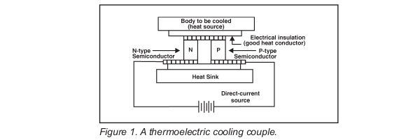
In 1834 Jean C. Peltier observed that, by passing an electric current through a junction of dissimilar metals, heat could be created or absorbed at the junction, depending on the direction of current fl ow. The Peltier effect, as it is now called, is the basis of all thermoelectric devices. Today thermoelectric cooling couples are generally made from two heavily doped semiconductor blocks (usually bismuth telluride), which are connected electrically in series and thermally in parallel, as shown in Figure 1. In this arrangement, heat absorbed at the cold junction is transferred to the hot junction at a rate proportional to the current passing through the couple. This effect is easily multiplied by increasing the number of couples used to form a thermoelectric module.

Conventional thermoelectric modules often contain dozens of thermoelectric cooling couples. The rate at which these modules can transfer heat from one surface to the other depends on the number of couples in the module, the current passing through the couples, the average temperature of the module and the temperature difference across it. An individual thermoelectric module may achieve a temperature differential as large as 60℃. However, to understand the practical performance characteristics of thermoelectric modules it is important to understand both internal and external limiting factors. In addition to the heat-pumping action of the Peltier effect, heat is also generated by the module and transferred through the module by conduction. In the absence of a thermal load, the maximum cooling-temperature differential is reached when the heat pumped by the Peltier effect is balanced by the other two factors. Fortunately, the performance graphs supplied by manufacturers of thermoelectric modules present the module performance in terms of the net of the internal factors. Figure 2 shows the performance of a typical module. The heat-transfer capability of the module drops to zero at a temperature differential of about 60℃.

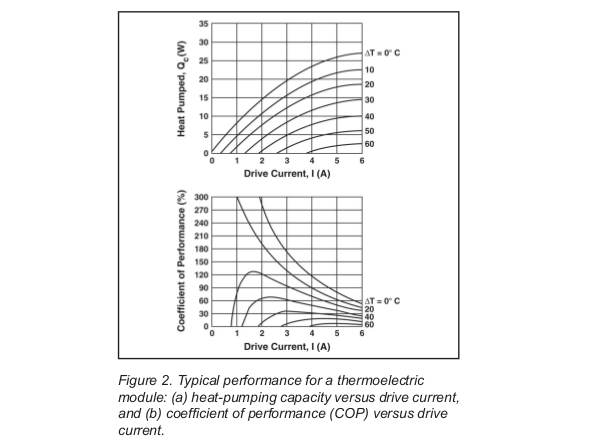
Figure 2 also shows how the module’s coefficient of performance (COP) varies with temperature differential and drive current. COP is defined as:

COP = (Heat transferred) ÷ (Total electrical power supplied) (1)

Remember, the heat that must be dissipated at the hot surface of the module includes both the heat removed from the cold surface and the joule heating caused by the power applied to the module. For example, using the data in Figure 2, we find that a drive current of about 4 A is required to pump 4 W across a temperature differential of 50℃. At this operating point, the module has a COP of about 17%, indicating that the total heat deposited at the hot surface of the module would be:

Q_total = Q_pumped × (1 + 1/COP) = 34 W (2)

External factors that limit heat-transfer performance include heat-sink limitations and also thermal-load considerations.

Heat Sink

Conceptually, the role of the heat sink is simple: to provide a constant-temperature surface, usually near room temperature. In some applications a large block of aluminum works well. However, when the heat to be dissipated exceeds about a watt, then fins, forced air or even fluid cooling are called for.

A 4” × 4” × 2” aluminum block at ambient temperature will heat up only about 5℃ in 10 minutes with 10 W being pumped into it. But over a period of an hour, it will continue to heat to about 23℃ above ambient. In contrast, a typical finned heat sink of roughly the same size will heat only about 12°C above ambient.

Thermal Load

In any application of thermoelectric cooling, the nature of the thermal load presented to the cooler and control circuit is critical. These loads can vary from a small diode-laser chip to a large focal-plane-detector array in an evacuated mount. Several important load parameters must be considered.

Thermal Mass - Thermal mass is the product of an object’s physical mass and specific heat. Large thermal mass is often a benefit when high stability is required, but it is a liability when rapid temperature change is needed. In a conventional 1300 nm, fiber-pigtailed diode laser package the internal thermoelectric cooler can change the laser chip temperature from room temperature to 0℃ in 2 or 3 seconds with the application of less than a watt of electrical power. However, to shift the temperature of the laser package itself over the same temperature range requires 40 seconds and the application of about 50 W

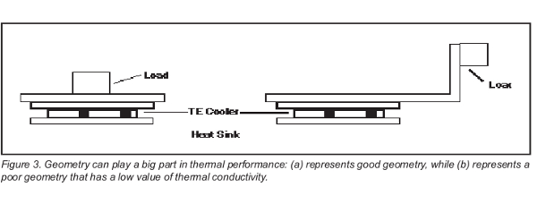
Geometry And Thermal Conductivity - To achieve optimum temperature control, the thermal path between the device to be cooled (or heated) and the face of the thermoelectric cooler should have high thermal conductivity and a short physical length. Figure 3 shows two simple arrangements that differ considerably in the ease with which they can be temperature-stabilized. The thermal connection between the load and cooler module in Figure 3b will exhibit low thermal conductivity and will introduce an undesirable delay factor. The low thermal conductivity will make the temperature at the load slow to respond to desired changes but highly susceptible to change induced by air currents. If active temperature control is used, the delay factor will lead to instability in the control loop, unless the loop gain is very low.

Also important is the quality of the contact between the faces of the cooler module and the surfaces they are attached to. Most manufacturers of thermoelectric cooler modules recommend that any gaps between these surfaces should be less than 0.001 inch.

In addition, a thin film of thermal Silicone grease (such as Corning® type 340 or Wake- type 340 or Wake- field® type 120) should be used between the type 120) should be used between the surfaces.

Device Heat Load - In many applications, In many applications, such as diode-laser temperature control, the device being cooled (or heated) produces heat itself. For example, a typical 3 mW diode laser will produce about 90 mW of heat when operated at room temperature. Under similar conditions, a 100 mW diode laser produces about 700 mW of heat.

Convective Heat Transfer - Convective Heat Transfer Naturally occurring Naturally occurring air currents cause thermal transfer between the heated (or cooled) device and the ambient surrounding air. The rate of transfer depends on the geometry of the load and its surroundings. This heat-transfer mechanism can become a limiting factor when the device must be cooled (or heated) far from ambient, as in some detector applications. In these cases an evacuated container is often used. For natural convection, heat will be transferred at a rate of about 0.5 to 1.0 mW/cm2 /℃. The following formula may be used to estimate heat transfer due to natural convection:

Q = h A (∆T) (3)

In this equation h = 0.5 to 1.0 mW/cm2 /℃, A is the surface area, and ∆T is the temperature difference between the cooled or heated surface and the surrounding ambient air. For example, a mounting plate 2 × 4 cm, which is cooled to 0℃, will absorb about 300 mW continuously from the surrounding 23℃ ambient air.

Conductive Heat Transfer - Any material connecting the thermal load to another surface provides a path for heat conduction. In most applications of thermoelectric coolers, the thermoelectric module itself is the largest conductive path. As discussed above, the effect of this path is generally accounted for in the performance data provided by the thermoelectric cooler manufacturer. However, the thermal conductivity of other paths, if any are present, must be included in calculating the total heat load. The appropriate equation is:

Q = k A ∆T/L (4)

where: k is the thermal conductivity (for aluminum k = 2.36 W/cm² /℃), A is the crosssectional area, L is the length and ∆T is the temperature difference.

Radiative Heat Transfer Radiative heat Radiative heat transfer varies as the fourth power of the temperature difference between the thermal load and its surroundings. Radiative heat transfer can be estimated using Equation 5, which assumes a small body (1) completely enclosed within a surrounding body (2):

Q = σ e₁ A₁ (T₁⁴ – T₂⁴) (5)

where σ is the Stephan-Boltzman constant, 5.67 × 10-8 W/m² /K, e₁ and A₁ are the emissivity and surface area of the enclosed body, and T₁ and T₂ are the absolute temperatures of the enclosed body and surrounding environment, respectively. For example, assuming a high-emissivity surface, a 1 cm² plate at 80℃ will lose 93 mW continuously to a 20℃ ambient surrounding. This loss drops to 12 mW if the plate is at 30℃. In either case the loss can be lowered considerably by reducing the surface emissivity of the plate. Gold coating, for example, will reduce the loss by a factor of about 50.

A practical example of thermoelectric temperature control is shown in Figure 4, which depicts a mechanical mounting fixture suitable for open-frame and window-can diode lasers. This mount offers a good compromise between mounting flexibility, speed with which temperature can be changed, and temperature stability.

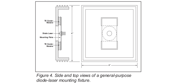
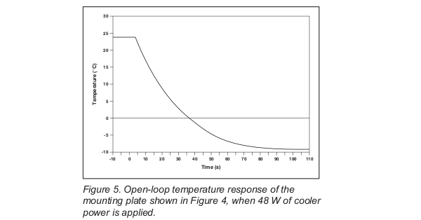
Figure 5 shows the open-loop response of the cooled mounting plate of this fi xture when 48 W of power is applied to the thermoelectric coolers.

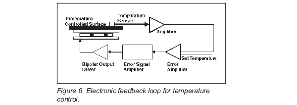
Precise, active temperature control with thermoelectric modules is usually accomplished with an electronic feedback loop such as the one shown in Figure 6. Key elements of this loop are the temperature sensor, error amplifier, error signal processor and bipolar output driver. The actual temperature is measured by the temperature sensor. This temperature is then compared to a set-point temperature, to produce an error signal proportional to the difference. The error signal processor produces an output based on the error signal and the control method being used. This output then controls a bipolar output driver, which is connected to the thermoelectric module. The complexity of this type of control loop varies from the simple analog proportional controllers found in most detector cooler controllers to fully digital PID (proportional-integral-differential) controllers.

Temperature Sensor - In most applications involving diode lasers or detectors, the temperature sensor is a negative-temperature- coefficient (NTC) thermistor. These devices offer several advantages; they are inexpensive, accurate, highly sensitive and easy to work with. Generally, their only disadvantage is that their resistance is a nonlinear function of temperature. However, this is not really a disadvantage if temperature control at a fixed point is required or when a microprocessor is available to perform the resistance-to-temperature conversion (and vice versa). In the latter case, the Steinhart-Hart equation can be used for thermistor calibration:

1÷T = A₀ + A₁ ln(R) + A₃ [ln(R)]³ (6)

In this equation T is the temperature in degrees Kelvin, R is the thermistor resistance in ohms, and A₀ , A₁ , and A₃ are the calibration constants. This equation can be used to calibrate most NTC thermistors to within 0.01℃ over a wide temperature range.

Other temperature sensors commonly used include semiconductor devices (such as the Analog Device AD590 or National Semiconductor LM335) and platinum Resistance Temperature Detectors (RTDs). These devices are linear but not as sensitive as thermistors.

Error Amplifier - The error amplifier amplifies The error amplifier amplifies the difference between the measured temperature (or thermistor resistance) and the set-point temperature (or resistance). This is usually accomplished with a simple operational-amplifier circuit.

Error Signal Processor - The error signal processor usually implements some form of the equation:

M = B + GE + (1/R) ∫E(s) ds + D (dE÷dt) (7)

In this equation M is the output of the error signal processor; B, G, R, and D are constants that depend on the thermal load and performance desired; and E represents the error signal input. The four terms on the right hand side of the equation represent a constant offset, a proportional term, an integral term, and a differential term.

Proportional Control

Most simple controllers implement only the proportional term of the equation:

M = GE (8)

In this case the drive signal to the thermoelectric module is proportional to the difference between the actual temperature (or thermistor resistance) and set-point temperature (or resistance). This type of controller is easily implemented using simple op-amp circuit elements. In practice the gain (G) of the circuit is set experimentally to produce a fast response with minimal overshoot to a step change in set point.

In proportional controllers there is always a residual error, even after the controller has settled to a final state. This error is proportional to difference between the set-point temperature and the actual temperature; it is inversely proportional to the gain of the controller loop. This is a particular problem when a large thermal load must be controlled. In this case the controller gain must be set low to prevent oscillation, but the low gain setting, in turn, leads to a large residual error.

Residual error can sometimes be mitigated by the addition of a constant offset (the first term in Equation 7). However, this is practical only in cases where the set-point and ambient temperatures remain relatively constant. Proportional controllers are usually a good choice only when the thermal load is small and tightly coupled to the thermoelectric cooler, or when only modest temperature stability is required. Examples include cooling detector and laser packages with internal TE coolers.

Proportional-Integral Control

Many of the problems of simple proportional controllers can be solved by adding the integral term of Equation 7. The integral removes any residual error. This advantage is not without cost, however, since a new parameter (R, often called the reset time of the controller) must be set. In some applications this can be a nuisance; to achieve optimum performance, both the loop gain, G, and reset time, R, must be adjusted each time the thermal load characteristics are changed.

In practice, it is often possible to select a single value of R and keep it constant while varying the loop gain, G, to accommodate differing thermal loads. Although performance is not optimum, it is usually acceptable and retains the inherent advantage of proportional-integral control.

The disadvantage of proportional-integral control is that the controller can be slow to integrate out large residual errors. This problem is overcome in full PID control loops.

Proportional-Integral-Differential (PID) Control

Full PID control loops implement all terms in Equation 7. The derivative term improves the loop’s response time by adding another parameter D. The differential parameter allows for effective handling of overshoot and ringing problems. This is very important when large thermal loads must be controlled quickly or rapid temperature cycling is important. ILX’s LDT-5948 and 5980 employ full PID control which allows them to control thermal loads rapidly and accurately.

Bipolar Output Driver - This stage simply This stage simply provides the power to drive the thermoelectric cooler modules. For power levels of a few watts, this function is easily accomplished using a bipolar transistor output stage. For power levels up to 120W, the LDT-5980 may be a wise choice for high power, rapid response, and highly accurate temperature control requirements.

Performance

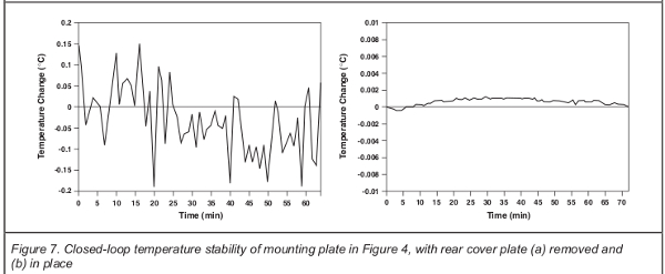
Two important performance criteria of temperature controllers are stability and speed. Under the right conditions, all three types of control architectures described above can achieve stabilities of better than 0.001℃. In practice, air currents in the vicinity of the load are usually the limiting factor for stability. Figure 7 shows the temperature fluctuation of the mounting plate in the fixture depicted in Figure 4, with and without the rear cover plate installed. In this example, active temperature control was performed with a proportional integral feedback loop. Further improvement could be obtained by using an insulating foam or glass wool inside the fixture, to further limit air currents.

The speed with which these control loops can respond to a step change in set temperature may vary depending on load characteristics and the amount of TE module power available. But as a reference point, we have found that it is practical to swing a standard fiber-pigtailed diode-laser package from room temperature to 0℃ in a period of less than 60 seconds.